Generating Tabular Synthetic Data Using GANs

Last updated on Dec 18, 2020 6 min read Deep Learning, GANs

Checkout mdedit.ai, AI powered Markdown Editor for tech writers

In this post, we will see how to generate tabular synthetic data using Generative adversarial networks(GANs). The goal is to generate synthetic data that is similar to the actual data in terms of statistics and demographics.

Introduction

It is important to ensure data privacy while publicly sharing information that contains sensitive information. There are numerous ways to tackle it and in this post we will use neural networks to generate synthetic data whose statistical features match the actual data.

We would be working with the Synthea dataset which is publicly available. Using the patients data from this dataset, we will try to generate synthetic data.

https://synthetichealth.github.io/synthea/

TL;DR

Checkout the Python Notebook if you are here just for the code.

https://colab.research.google.com/drive/1vBnSrTP8liPlnGg5ArzUk08oDLnERDbF?usp=sharing

Data Preprocessing

Firstly, download the publicly available synthea dataset and unzip it.

	!wget https://storage.googleapis.com/synthea-public/synthea_sample_data_csv_apr2020.zip
	!unzip synthea_sample_data_csv_apr2020.zip

view raw bfcd3153-113d-4520-abd5-7e51a35cacff hosted with ❤ by GitHub

Remove unnecessary columns and encode all data

Next, read patients data and remove fields such as id, date, SSN, name etc. Note, that we are trying to generate synthetic data which can be used to train our deep learning models for some other tasks. For such a model, we don’t require fields like id, date, SSN etc.

	import pandas as pd

	df = pd.read_csv('csv/patients.csv')
	df.drop(['Id', 'BIRTHDATE', 'DEATHDATE', 'SSN', 'DRIVERS', 'PASSPORT', 'PREFIX',
	'FIRST', 'ADDRESS', 'LAST', 'SUFFIX', 'MAIDEN','LAT', 'LON',], axis=1, inplace=True)
	print(df.columns)

view raw 1613e49a-a7f8-4753-bca6-84140400fec8 hosted with ❤ by GitHub

Index(['MARITAL', 'RACE', 'ETHNICITY', 'GENDER', 'BIRTHPLACE', 'CITY', 'STATE',
       'COUNTY', 'ZIP', 'HEALTHCARE_EXPENSES', 'HEALTHCARE_COVERAGE'],
      dtype='object')

Next, we will encode all categorical features to integer values. We are simply encoding the features to numerical values and are not using one hot encoding as its not required for GANs.

	df["MARITAL"] = df["MARITAL"].astype('category').cat.codes
	df["RACE"] = df["RACE"].astype('category').cat.codes
	df["ETHNICITY"] = df["ETHNICITY"].astype('category').cat.codes
	df["GENDER"] = df["GENDER"].astype('category').cat.codes
	df["BIRTHPLACE"] = df["BIRTHPLACE"].astype('category').cat.codes
	df["CITY"] = df["CITY"].astype('category').cat.codes
	df["STATE"] = df["STATE"].astype('category').cat.codes
	df["COUNTY"] = df["COUNTY"].astype('category').cat.codes
	df["ZIP"] = df["ZIP"].astype('category').cat.codes

	df.head()

view raw 6edf7e46-5cea-4c2e-aab3-4c22fa8a48a1 hosted with ❤ by GitHub

	MARITAL	RACE	ETHNICITY	GENDER	BIRTHPLACE	CITY	COUNTY	ZIP	HEALTHCARE_EXPENSES	HEALTHCARE_COVERAGE
0	0	4	0	1	136	42	6	2	271227.08	1334.88
1	0	4	1	1	61	186	8	132	793946.01	3204.49
2	0	4	1	1	236	42	6	3	574111.90	2606.40
3	0	4	1	0	291	110	8	68	935630.30	8756.19
4	-1	4	1	1	189	24	12	125	598763.07	3772.20

Next, we will encode all continious features to equally sized bins. First, lets find the minimum and maximum values for HEALTHCARE_EXPENSES and HEALTHCARE_COVERAGE and then create bins based on these values.

	HEALTHCARE_EXPENSES_MIN = df["HEALTHCARE_EXPENSES"].min()
	HEALTHCARE_EXPENSES_MAX = df["HEALTHCARE_EXPENSES"].max()
	print('Min and max healthcare expense', HEALTHCARE_EXPENSES_MIN, HEALTHCARE_EXPENSES_MAX)

	HEALTHCARE_COVERAGE_MIN = df["HEALTHCARE_COVERAGE"].min()
	HEALTHCARE_COVERAGE_MAX = df["HEALTHCARE_COVERAGE"].max()

	print('Min and max healthcare coverage', HEALTHCARE_COVERAGE_MIN, HEALTHCARE_COVERAGE_MAX)

view raw fe23fec7-44f3-4268-81df-0af2da4fca76 hosted with ❤ by GitHub

Min and max healthcare expense 1822.1600000000005 2145924.400000002
Min and max healthcare coverage 0.0 927873.5300000022

Now, we encode HEALTHCARE_EXPENSES and HEALTHCARE_COVERAGE into bins using the pd.cut method. We use numpy’s linspace method to create equally sized bins.

	import numpy as np

	df_healthcare_expenses = pd.cut(df['HEALTHCARE_EXPENSES'], bins=np.linspace(HEALTHCARE_EXPENSES_MIN, HEALTHCARE_EXPENSES_MAX, 21), labels=False)
	df_healthcare_coverage = pd.cut(df['HEALTHCARE_COVERAGE'], bins=np.linspace(HEALTHCARE_COVERAGE_MIN, HEALTHCARE_COVERAGE_MAX, 21), labels=False)

	df.drop(["HEALTHCARE_EXPENSES", "HEALTHCARE_COVERAGE"], axis=1, inplace=True)

	df = pd.concat([df, df_healthcare_expenses, df_healthcare_coverage], axis=1)

view raw 21570e62-78ff-4e23-b5ec-4fc22fa3b476 hosted with ❤ by GitHub

Transform the data

Next, we apply PowerTransformer on all the fields to get a Gaussian distribution for the data.

	from sklearn.preprocessing import PowerTransformer

	df[df.columns] = PowerTransformer(method='yeo-johnson', standardize=True, copy=True).fit_transform(df[df.columns])

	print(df)

view raw 380d3c1c-b010-42e0-a2ce-5310e4169588 hosted with ❤ by GitHub

       MARITAL      RACE  ...  HEALTHCARE_EXPENSES  HEALTHCARE_COVERAGE
0     0.334507  0.461541  ...            -0.819522            -0.187952
1     0.334507  0.461541  ...             0.259373            -0.187952
2     0.334507  0.461541  ...            -0.111865            -0.187952
3     0.334507  0.461541  ...             0.426979            -0.187952
4    -1.275676  0.461541  ...            -0.111865            -0.187952
...        ...       ...  ...                  ...                  ...
1166  0.334507 -2.207146  ...             1.398831            -0.187952
1167  1.773476  0.461541  ...             0.585251            -0.187952
1168  1.773476  0.461541  ...             1.275817             5.320497
1169  0.334507  0.461541  ...             1.016430            -0.187952
1170  0.334507  0.461541  ...             1.275817            -0.187952

[1171 rows x 11 columns]


/usr/local/lib/python3.6/dist-packages/sklearn/preprocessing/_data.py:2982: RuntimeWarning: divide by zero encountered in log
  loglike = -n_samples / 2 * np.log(x_trans.var())

Train the Model

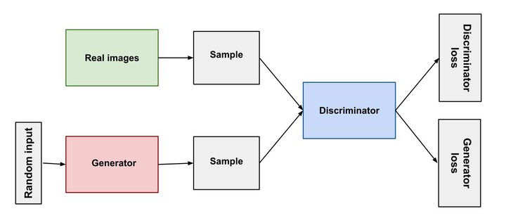
Next, lets define the neural network for generating synthetic data. We will be using a GAN network that comprises of an generator and discriminator that tries to beat each other and in the process learns the vector embedding for the data.

The model was taken from a Github repository where it is used to generate synthetic data on credit card fraud data.

	import os
	import numpy as np

	import tensorflow as tf
	from tensorflow.keras.layers import Input, Dense, Dropout
	from tensorflow.keras import Model

	from tensorflow.keras.optimizers import Adam

	class GAN():

	def __init__(self, gan_args):
	[self.batch_size, lr, self.noise_dim,
	self.data_dim, layers_dim] = gan_args

	self.generator = Generator(self.batch_size).\
	build_model(input_shape=(self.noise_dim,), dim=layers_dim, data_dim=self.data_dim)

	self.discriminator = Discriminator(self.batch_size).\
	build_model(input_shape=(self.data_dim,), dim=layers_dim)

	optimizer = Adam(lr, 0.5)

	# Build and compile the discriminator
	self.discriminator.compile(loss='binary_crossentropy',
	optimizer=optimizer,
	metrics=['accuracy'])

	# The generator takes noise as input and generates imgs
	z = Input(shape=(self.noise_dim,))
	record = self.generator(z)

	# For the combined model we will only train the generator
	self.discriminator.trainable = False

	# The discriminator takes generated images as input and determines validity
	validity = self.discriminator(record)

	# The combined model (stacked generator and discriminator)
	# Trains the generator to fool the discriminator
	self.combined = Model(z, validity)
	self.combined.compile(loss='binary_crossentropy', optimizer=optimizer)

	def get_data_batch(self, train, batch_size, seed=0):
	# # random sampling - some samples will have excessively low or high sampling, but easy to implement
	# np.random.seed(seed)
	# x = train.loc[ np.random.choice(train.index, batch_size) ].values
	# iterate through shuffled indices, so every sample gets covered evenly

	start_i = (batch_size * seed) % len(train)
	stop_i = start_i + batch_size
	shuffle_seed = (batch_size * seed) // len(train)
	np.random.seed(shuffle_seed)
	train_ix = np.random.choice(list(train.index), replace=False, size=len(train)) # wasteful to shuffle every time
	train_ix = list(train_ix) + list(train_ix) # duplicate to cover ranges past the end of the set
	x = train.loc[train_ix[start_i: stop_i]].values
	return np.reshape(x, (batch_size, -1))

	def train(self, data, train_arguments):
	[cache_prefix, epochs, sample_interval] = train_arguments

	data_cols = data.columns

	# Adversarial ground truths
	valid = np.ones((self.batch_size, 1))
	fake = np.zeros((self.batch_size, 1))

	for epoch in range(epochs):
	# ---------------------
	# Train Discriminator
	# ---------------------
	batch_data = self.get_data_batch(data, self.batch_size)
	noise = tf.random.normal((self.batch_size, self.noise_dim))

	# Generate a batch of new images
	gen_data = self.generator.predict(noise)

	# Train the discriminator
	d_loss_real = self.discriminator.train_on_batch(batch_data, valid)
	d_loss_fake = self.discriminator.train_on_batch(gen_data, fake)
	d_loss = 0.5 * np.add(d_loss_real, d_loss_fake)

	# ---------------------
	# Train Generator
	# ---------------------
	noise = tf.random.normal((self.batch_size, self.noise_dim))
	# Train the generator (to have the discriminator label samples as valid)
	g_loss = self.combined.train_on_batch(noise, valid)

	# Plot the progress
	print("%d [D loss: %f, acc.: %.2f%%] [G loss: %f]" % (epoch, d_loss[0], 100 * d_loss[1], g_loss))

	# If at save interval => save generated events
	if epoch % sample_interval == 0:
	#Test here data generation step
	# save model checkpoints
	model_checkpoint_base_name = 'model/' + cache_prefix + '_{}_model_weights_step_{}.h5'
	self.generator.save_weights(model_checkpoint_base_name.format('generator', epoch))
	self.discriminator.save_weights(model_checkpoint_base_name.format('discriminator', epoch))

	#Here is generating the data
	z = tf.random.normal((432, self.noise_dim))
	gen_data = self.generator(z)
	print('generated_data')

	def save(self, path, name):
	assert os.path.isdir(path) == True, \
	"Please provide a valid path. Path must be a directory."
	model_path = os.path.join(path, name)
	self.generator.save_weights(model_path) # Load the generator
	return

	def load(self, path):
	assert os.path.isdir(path) == True, \
	"Please provide a valid path. Path must be a directory."
	self.generator = Generator(self.batch_size)
	self.generator = self.generator.load_weights(path)
	return self.generator

	class Generator():
	def __init__(self, batch_size):
	self.batch_size=batch_size

	def build_model(self, input_shape, dim, data_dim):
	input= Input(shape=input_shape, batch_size=self.batch_size)
	x = Dense(dim, activation='relu')(input)
	x = Dense(dim * 2, activation='relu')(x)
	x = Dense(dim * 4, activation='relu')(x)
	x = Dense(data_dim)(x)
	return Model(inputs=input, outputs=x)

	class Discriminator():
	def __init__(self,batch_size):
	self.batch_size=batch_size

	def build_model(self, input_shape, dim):
	input = Input(shape=input_shape, batch_size=self.batch_size)
	x = Dense(dim * 4, activation='relu')(input)
	x = Dropout(0.1)(x)
	x = Dense(dim * 2, activation='relu')(x)
	x = Dropout(0.1)(x)
	x = Dense(dim, activation='relu')(x)
	x = Dense(1, activation='sigmoid')(x)
	return Model(inputs=input, outputs=x)

view raw d40a0881-57b1-4fcc-acb5-2589f202a63e hosted with ❤ by GitHub

Next, lets define the training parameters for the GAN network. We would be using a batch size of 32 and train it for 5000 epochs.

data_cols = df.columns

view raw 9495771c-3a9c-4ef9-9454-8dbeec5e9bed hosted with ❤ by GitHub

	#Define the GAN and training parameters
	noise_dim = 32
	dim = 128
	batch_size = 32

	log_step = 100
	epochs = 5000+1
	learning_rate = 5e-4
	models_dir = 'model'

	df[data_cols] = df[data_cols]

	print(df.shape[1])

	gan_args = [batch_size, learning_rate, noise_dim, df.shape[1], dim]
	train_args = ['', epochs, log_step]

view raw 77aef765-9f93-4bd2-9069-8bc0002a8035 hosted with ❤ by GitHub

!mkdir model

view raw 0ffb34fa-345e-4c57-b652-269b7de763c6 hosted with ❤ by GitHub

mkdir: cannot create directory ‘model’: File exists

Finally, let’s run the training and see if the model is able to learn something.

	model = GAN

	#Training the GAN model chosen: Vanilla GAN, CGAN, DCGAN, etc.
	synthesizer = model(gan_args)
	synthesizer.train(df, train_args)

view raw c4ce65cb-5432-480b-b7ad-e01934a4b5f8 hosted with ❤ by GitHub

[1;30;43mStreaming output truncated to the last 5000 lines.[0m
generated_data
101 [D loss: 0.324169, acc.: 85.94%] [G loss: 2.549267]
.
.
.
4993 [D loss: 0.150710, acc.: 95.31%] [G loss: 2.865143]
4994 [D loss: 0.159454, acc.: 95.31%] [G loss: 2.886763]
4995 [D loss: 0.159046, acc.: 95.31%] [G loss: 2.640226]
4996 [D loss: 0.150796, acc.: 95.31%] [G loss: 2.868319]
4997 [D loss: 0.170520, acc.: 95.31%] [G loss: 2.697939]
4998 [D loss: 0.161605, acc.: 95.31%] [G loss: 2.601780]
4999 [D loss: 0.156147, acc.: 95.31%] [G loss: 2.719781]
5000 [D loss: 0.164568, acc.: 95.31%] [G loss: 2.826339]
WARNING:tensorflow:Model was constructed with shape (32, 32) for input Tensor("input_1:0", shape=(32, 32), dtype=float32), but it was called on an input with incompatible shape (432, 32).
generated_data

After, 5000 epochs the models shows a training accuracy of 95.31% which sounds quite impressive.

	!mkdir model/gan
	!mkdir model/gan/saved

view raw cfa0be5e-765f-49f8-beec-e8b49ab4a6d1 hosted with ❤ by GitHub

mkdir: cannot create directory ‘model/gan’: File exists
mkdir: cannot create directory ‘model/gan/saved’: File exists

	#You can easily save the trained generator and loaded it aftwerwards

	synthesizer.save('model/gan/saved', 'generator_patients')

view raw 3c874d03-5943-4e36-8eae-fe0a2f3666ff hosted with ❤ by GitHub

Let’s take a look at the Generator and Discriminator models.

synthesizer.generator.summary()

view raw bb1b29d4-f902-4cc6-8a27-7598a97d01b3 hosted with ❤ by GitHub

Model: "model"
_________________________________________________________________
Layer (type)                 Output Shape              Param #   
=================================================================
input_1 (InputLayer)         [(32, 32)]                0         
_________________________________________________________________
dense (Dense)                (32, 128)                 4224      
_________________________________________________________________
dense_1 (Dense)              (32, 256)                 33024     
_________________________________________________________________
dense_2 (Dense)              (32, 512)                 131584    
_________________________________________________________________
dense_3 (Dense)              (32, 11)                  5643      
=================================================================
Total params: 174,475
Trainable params: 174,475
Non-trainable params: 0
_________________________________________________________________

synthesizer.discriminator.summary()

view raw 33493005-b6d5-4c15-ae3a-03902961245a hosted with ❤ by GitHub

Model: "model_1"
_________________________________________________________________
Layer (type)                 Output Shape              Param #   
=================================================================
input_2 (InputLayer)         [(32, 11)]                0         
_________________________________________________________________
dense_4 (Dense)              (32, 512)                 6144      
_________________________________________________________________
dropout (Dropout)            (32, 512)                 0         
_________________________________________________________________
dense_5 (Dense)              (32, 256)                 131328    
_________________________________________________________________
dropout_1 (Dropout)          (32, 256)                 0         
_________________________________________________________________
dense_6 (Dense)              (32, 128)                 32896     
_________________________________________________________________
dense_7 (Dense)              (32, 1)                   129       
=================================================================
Total params: 170,497
Trainable params: 0
Non-trainable params: 170,497
_________________________________________________________________

Evaluation

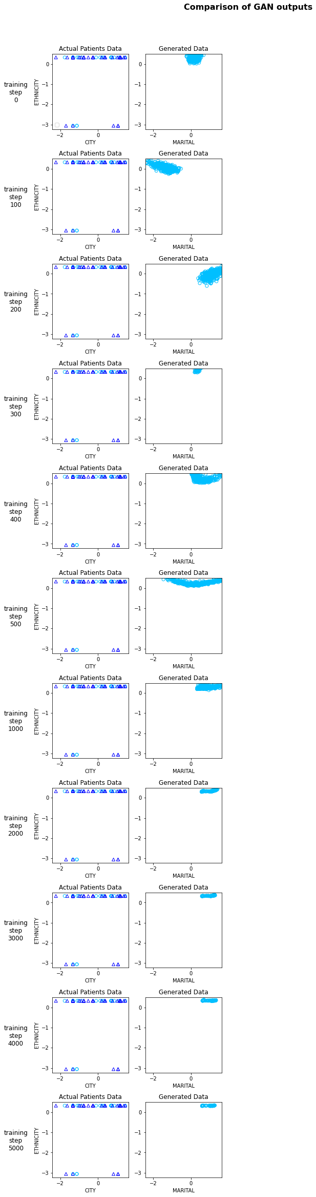
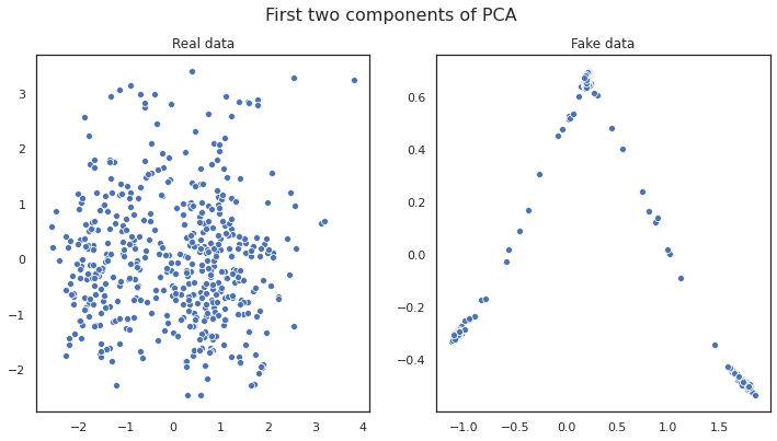
Now, that we have trained the model let’s see if the generated data is similar to the actual data.

We plot the generated data for some of the model steps and see how the plot for the generated data changes as the networks learns the embedding more accurately.

models = {'GAN': ['GAN', False, synthesizer.generator]}

view raw 01d2a4d1-d1e7-4ead-b521-0cd02c73f11d hosted with ❤ by GitHub

	import matplotlib.pyplot as plt

	# Setup parameters visualization parameters
	seed = 17
	test_size = 492 # number of fraud cases
	noise_dim = 32

	np.random.seed(seed)
	z = np.random.normal(size=(test_size, noise_dim))
	real = synthesizer.get_data_batch(train=df, batch_size=test_size, seed=seed)
	real_samples = pd.DataFrame(real, columns=data_cols)

	model_names = ['GAN']
	colors = ['deepskyblue','blue']
	markers = ['o','^']

	col1, col2 = 'CITY', 'ETHNICITY'

	base_dir = 'model/'

	#Actual fraud data visualization
	model_steps = [ 0, 100, 200, 300, 400, 500, 1000, 2000, 3000, 4000, 5000]
	rows = len(model_steps)
	columns = 5

	axarr = [[]]*len(model_steps)

	fig = plt.figure(figsize=(14,rows*3))

	for model_step_ix, model_step in enumerate(model_steps):
	axarr[model_step_ix] = plt.subplot(rows, columns, model_step_ix*columns + 1)

	for group, color, marker in zip(real_samples.groupby('RACE'), colors, markers):
	plt.scatter( group[1][[col1]], group[1][[col2]], marker=marker, edgecolors=color, facecolors='none' )

	plt.title('Actual Patients Data')
	plt.ylabel(col2) # Only add y label to left plot
	plt.xlabel(col1)
	xlims, ylims = axarr[model_step_ix].get_xlim(), axarr[model_step_ix].get_ylim()

	if model_step_ix == 0:
	legend = plt.legend()
	legend.get_frame().set_facecolor('white')

	i=0
	[model_name, with_class, generator_model] = models['GAN']

	generator_model.load_weights( base_dir + '_generator_model_weights_step_'+str(model_step)+'.h5')

	ax = plt.subplot(rows, columns, model_step_ix*columns + 1 + (i+1) )

	g_z = generator_model.predict(z)
	gen_samples = pd.DataFrame(g_z, columns=data_cols)
	gen_samples.to_csv('Generated_sample.csv')
	plt.scatter( gen_samples[[col1]], gen_samples[[col2]], marker=markers[0], edgecolors=colors[0], facecolors='none' )
	plt.title("Generated Data")
	plt.xlabel(data_cols[0])
	ax.set_xlim(xlims), ax.set_ylim(ylims)

	plt.suptitle('Comparison of GAN outputs', size=16, fontweight='bold')
	plt.tight_layout(rect=[0.075,0,1,0.95])

	# Adding text labels for traning steps
	vpositions = np.array([ i._position.bounds[1] for i in axarr ])
	vpositions += ((vpositions[0] - vpositions[1]) * 0.35 )
	for model_step_ix, model_step in enumerate( model_steps ):
	fig.text( 0.05, vpositions[model_step_ix], 'training\nstep\n'+str(model_step), ha='center', va='center', size=12)

	plt.savefig('Comparison_of_GAN_outputs.png')

view raw 94cdb64a-8e7b-4a0f-be7b-7ef837d947d3 hosted with ❤ by GitHub

No handles with labels found to put in legend.

png

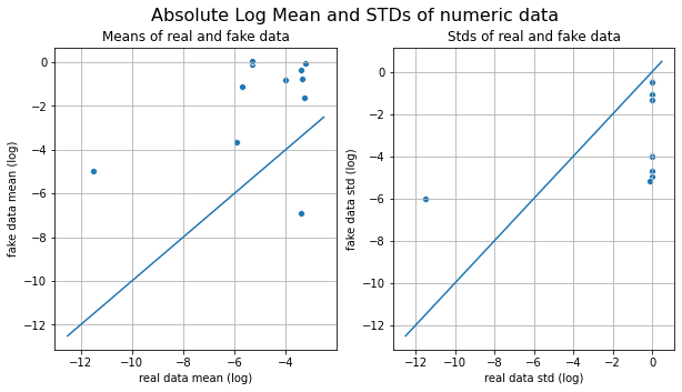
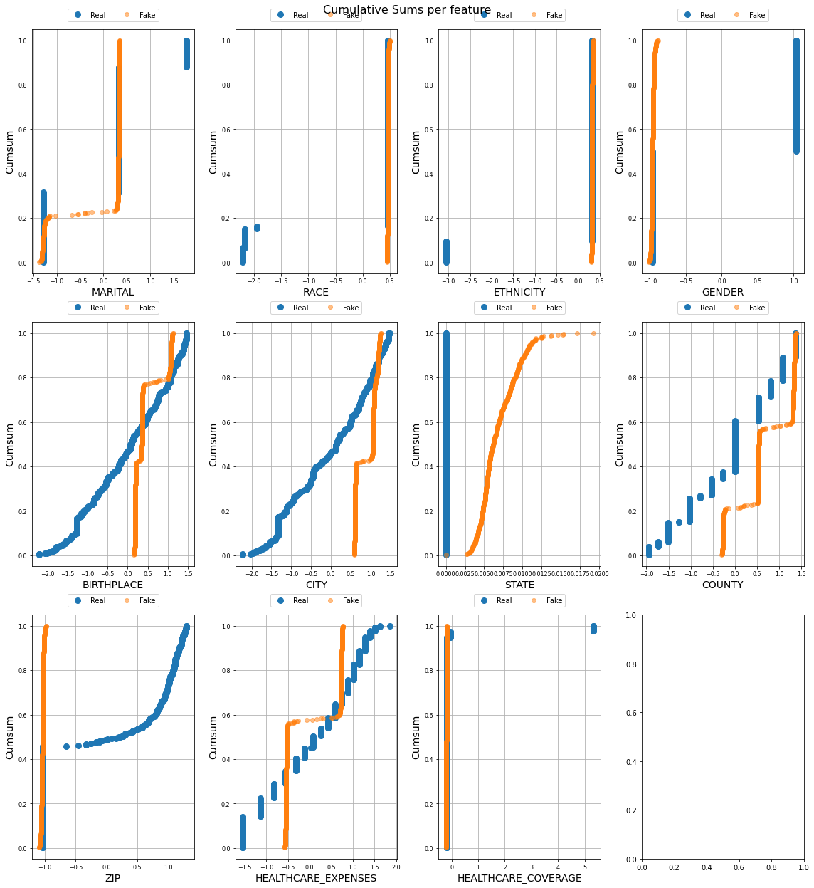
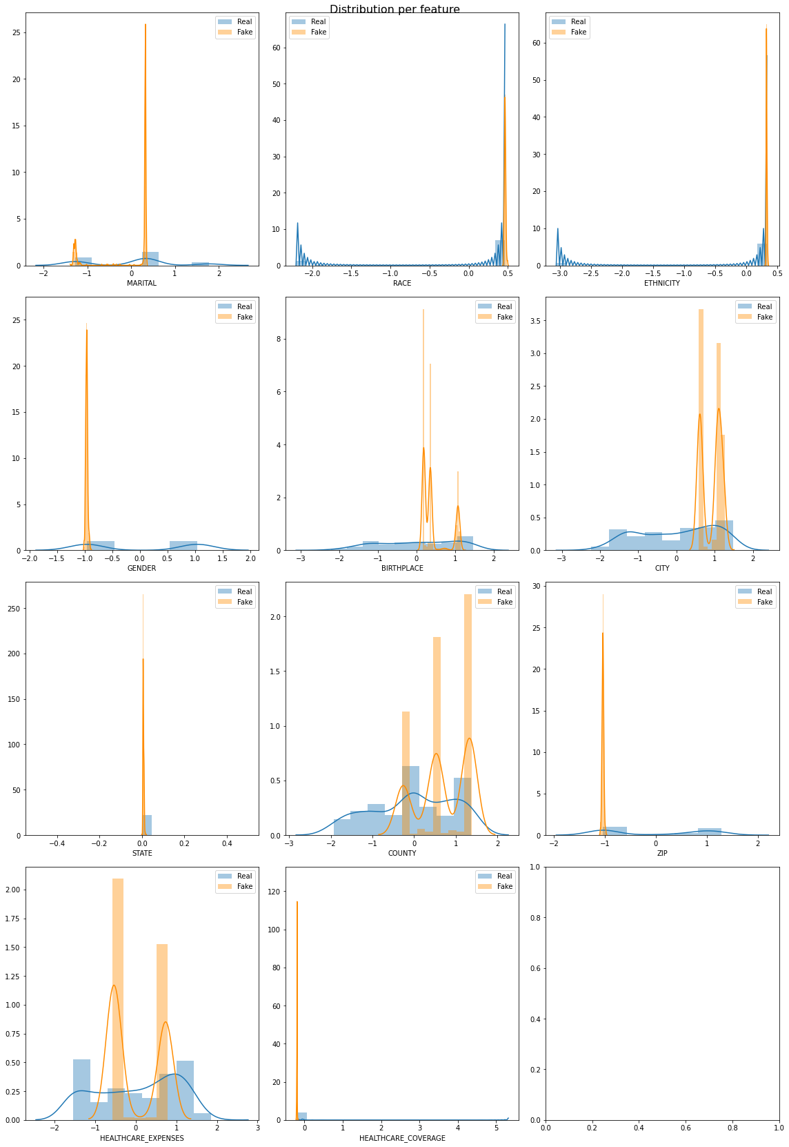
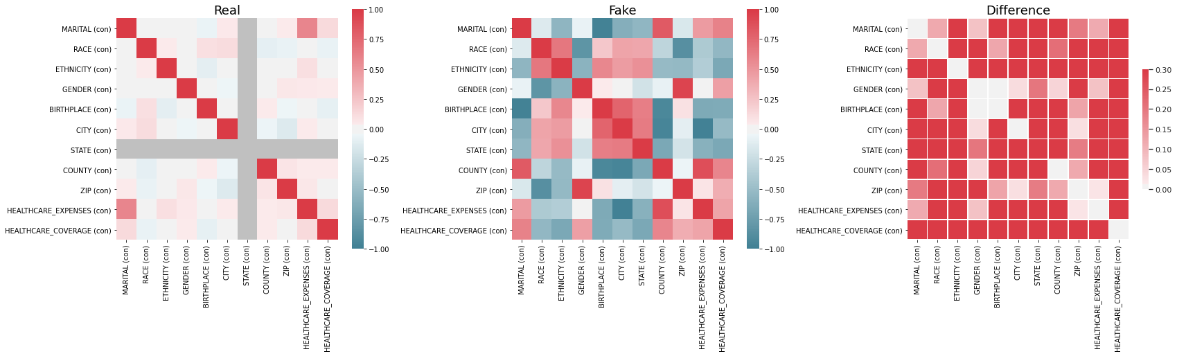
Now let’s try to do a feature by feature comparision between the generated data and the actual data. We will use python’s table_evaluator library to compare the features.

	!pip install table_evaluator

view raw 49895f08-0feb-4a82-9ecc-5776bbb40dec hosted with ❤ by GitHub

	gen_df.drop('Unnamed: 0', axis=1, inplace=True)
	print(gen_df.columns)
	print(df.shape, gen_df.shape)

view raw edd86a78-41b2-4bc6-9f8b-e3e148c879fb hosted with ❤ by GitHub

Index(['MARITAL', 'RACE', 'ETHNICITY', 'GENDER', 'BIRTHPLACE', 'CITY', 'STATE',
       'COUNTY', 'ZIP', 'HEALTHCARE_EXPENSES', 'HEALTHCARE_COVERAGE'],
      dtype='object')
(1171, 11) (492, 11)

We call the visual_evaluation method to compare the actual date(df) and the generated data(gen_df).

	from table_evaluator import load_data, TableEvaluator

	cat_cols = ['MARITAL', 'RACE', 'ETHNICITY', 'GENDER', 'BIRTHPLACE', 'CITY', 'STATE', 'COUNTY', 'ZIP']

	print(len(df), len(gen_df))
	table_evaluator = TableEvaluator(df, gen_df)

	table_evaluator.visual_evaluation()

view raw 468e12a0-e57b-4c98-9f88-158d5bb2dad4 hosted with ❤ by GitHub

1171 492

png

/usr/local/lib/python3.6/dist-packages/seaborn/distributions.py:283: UserWarning: Data must have variance to compute a kernel density estimate.
  warnings.warn(msg, UserWarning)

png

Conclusion

Some of the features in the syntehtic data match closely with actual data but there are some other features which were not learnt perfectly by the model. We can keep playing with the model and its hyperparameters to improve the model further.

This post demonstrates that its fairly simply to use GANs to generate synthetic data where the actual data is sensitive in nature and can’t be shared publicly.

Deep Learning GANs Privacy Synthetic Data