Analyzing Bike Sharing Demand

Last updated on Feb 12, 2021 10 min read Data Science

Recently, I worked on an assignment to analyze the data from bikesharing system to predict its demand. In this post, we will see how the given data can be analyzed using statistical machine learning methods.

The original dataset can be found here on Kaggle.

https://www.kaggle.com/c/bike-sharing-demand

In this notebook, we would be using a small subset of this dataset and just focus on the methodology. The accuracies can’t be expected to be high for such a small subset of the dataset. Feel free to use the complete dataset for your analysis.

You can download the CSV data used in this noteboot from Google drive.

https://drive.google.com/file/d/1GWbrrsPe6B-0ZKn4Dxd7D8pNvfK6IsQZ/view?usp=sharing

	from google.colab import drive

	drive.mount('/content/gdrive')

view raw b8865f6a-0b4c-4254-b044-ab5419130800 hosted with ❤ by GitHub

	import pandas as pd

	bikeshare_df = pd.read_csv("/content/gdrive/My Drive/cv_data/jpmc/Bikeshare_data.csv")

	print(bikeshare_df.head())

view raw 9dab9362-3c1c-4b67-a19d-42d244a0f380 hosted with ❤ by GitHub

   season month  holiday day_of_week  ...  atemp humidity  windspeed   count
0  Spring   May        0         Tue  ...   26.0  76.5833   0.118167  6073.0
1    Fall   Dec        0         Tue  ...   19.0  73.3750   0.174129  6606.0
2  Spring   Jun        0         Thu  ...   28.0  56.9583   0.253733  7363.0
3    Fall   Dec        0         Sun  ...    4.0  58.6250   0.169779  2431.0
4  Summer   Sep        0         Wed  ...   23.0  91.7083   0.097021  1996.0

[5 rows x 11 columns]

Data Exploration

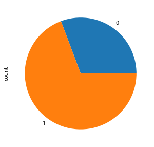
Bikeshares for weekend vs weekdays

The plot uses the workingday column to get information about weekday or weekend. Clearly lot more bikeshares happen on weekdays as compared to weekends.

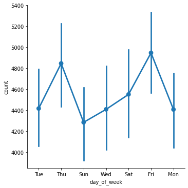
Also, on a more detailed level the factor plot is plotted to see the variations in bikeshares based on the day of the week.

The factor plot reaffirms our observation from the pie chart and tells us that during weekends Sunday sees the least number of bikeshares.

	import seaborn as sns
	import matplotlib.pyplot as plt

	plt.figure(figsize=(5,5))
	bikeshare_df.groupby(["workingday"])["count"].sum().plot.pie()

view raw 44b0b8ea-22a1-4da3-823a-c5887e5a57de hosted with ❤ by GitHub

png

	g = sns.factorplot(data = bikeshare_df,
	x = "day_of_week",
	y = "count",
	ci = 95
	)

view raw e8d77c5c-591b-4cef-8e44-10f7aab5bc97 hosted with ❤ by GitHub

png

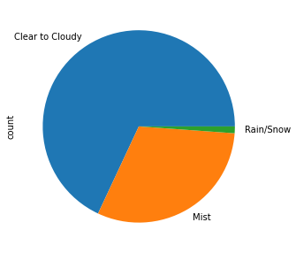
Bikeshares during different weather conditions

The plot below shows that most bikeshares happen when the weather is clear to cloudy. People also seem to be using bikeshares in misty weather conditions. Quite intuitively, the number of bikeshares on a rainy or snowy day is quite less.

	plt.figure(figsize=(5,5))
	bikeshare_df.groupby(["weather"])["count"].sum().plot.pie()

view raw 9007c9ea-5f9b-4bb6-89b5-90a07d30a5e0 hosted with ❤ by GitHub

png

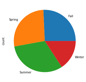
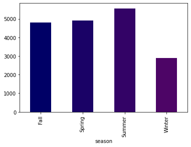
Bikeshares during different seasons

Firstly a pie chart is plotted for visualizing the number of bikeshares in different seasons. The pie chart doesn’t provide a clear picture so next a bar chart is used to get a clearer picture.

The bar chart shows that most bikeshares happen during Summer while Winter accounts for the least number of bikeshares.

	plt.figure(figsize=(5,5))
	bikeshare_df.groupby(["season"])["count"].sum().plot.pie()

view raw 4983399d-3f68-4f8f-b662-0e5cbc1fe1c2 hosted with ❤ by GitHub

png

	my_colors = [(x/10, x/150.0, 0.4) for x in range(5)]
	bikeshare_df.groupby("season")["count"].mean().plot.bar(color =my_colors)

view raw f914e930-0033-4575-a56a-d24c9e0c39a1 hosted with ❤ by GitHub

png

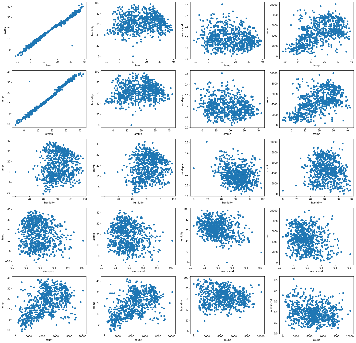
Exploring linear non-linear dependencies

As it is apparent from the plots below, some of the variables have linear dependencies with others while some don’t have a linear relationship.

Variable	Linear	Inverse-linear	Non-Linear
Temp	atemp, count	-	humidity, windspeed
atemp	temp, count	-	humidity, windspeed
humidity	-	windspeed	temp, atemp, count
windspeed	-	humidity	temp, atemp, count
count	temp, atemp	-	humidity, windspeed

	import matplotlib.pyplot as plt
	import statsmodels.api as sm

	fig, axes = plt.subplots(nrows=5, ncols=4, figsize=(25,25))

	columns = ['temp', 'atemp', 'humidity', 'windspeed', 'count']

	ax= axes.flatten()

	idx = 0
	for i, val1 in enumerate(columns):
	for j, val2 in enumerate(columns):
	if val1!=val2:
	ax[idx].scatter(bikeshare_df[val1], bikeshare_df[val2])
	ax[idx].set_xlabel(val1)
	ax[idx].set_ylabel(val2)
	idx+=1

	plt.show()

view raw 8abf0437-3225-4590-af16-8c68ab6444a7 hosted with ❤ by GitHub

png

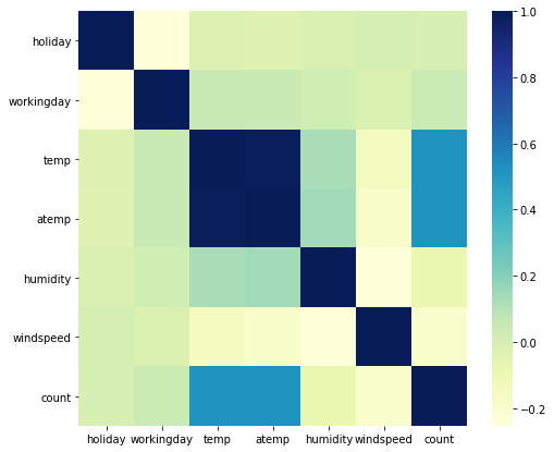
Moreover, lets find the correlation between the variables to further analyse the dependencies between variables.

In the correlation heatmap, the blue shades represent higher level of correlation between the variables.

Note: temp, atemp variables show good amount of positive correlation with count.

	print(bikeshare_df.columns)
	corr = bikeshare_df.corr(method='pearson')
	plt.figure(figsize = (8,7))

	g = sns.heatmap(corr,
	xticklabels=corr.columns.values,
	yticklabels=corr.columns.values, cmap="YlGnBu")

view raw 9266803d-3877-4f5a-8ee8-f8014a26d089 hosted with ❤ by GitHub

Index(['season', 'month', 'holiday', 'day_of_week', 'workingday', 'weather',
       'temp', 'atemp', 'humidity', 'windspeed', 'count'],
      dtype='object')

png

Should polynomial transformation be performed?

Clearly not all features exhibit a linear dependency with the predictor variable ie. count so it might be worthwhile to try a polynomial transformation and visualize the dependencies again.

Before that lets do some more data exploration to further improve the data for linear regression.

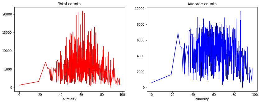
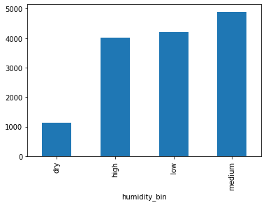
Bikeshares sum and mean plots grouped based on humidity

The idea is to see the variations in bikeshares for different humidity levels and then bin the values into multiple groups.

	plt.figure(figsize= (14,5))

	plt.subplot(1,2,1)
	bikeshare_df.groupby("humidity")["count"].sum().plot(color="r")
	plt.title("Total counts")

	plt.subplot(1,2,2)
	bikeshare_df.groupby("humidity")["count"].mean().plot(color="b")
	plt.title("Average counts")

view raw 78b09cbe-25f4-4f14-b152-331ee4fdfa49 hosted with ❤ by GitHub

Text(0.5, 1.0, 'Average counts')

png

	bikeshare_df["humidity_bin"] = pd.cut(bikeshare_df["humidity"],4, labels= ["dry", "low", "medium", "high"])

	# drop the original column
	bikeshare_df.drop(['humidity'], axis=1, inplace=True)

	bikeshare_df.groupby("humidity_bin")["count"].mean().sort_values().plot.bar()

view raw 46ffad39-fcd0-46e8-ac6c-b716fbf55768 hosted with ❤ by GitHub

png

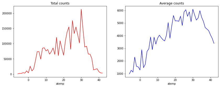
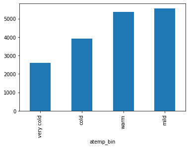
Bikeshares sum and mean plots grouped based on atemp

Similar to humidity, the idea is to see the variations in bikeshares for different atemp levels and then bin the values into multiple groups.

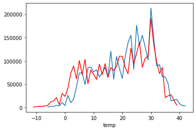
Moreover, temp and atemp is compared to see how these values vary.

	plt.figure(figsize= (14,5))

	plt.subplot(1,2,1)
	bikeshare_df.groupby("atemp")["count"].sum().plot(color="r")
	plt.title("Total counts")

	plt.subplot(1,2,2)
	bikeshare_df.groupby("atemp")["count"].mean().plot(color="b")
	plt.title("Average counts")

view raw 0bf03b43-7e64-4036-8857-659b2223fb48 hosted with ❤ by GitHub

Text(0.5, 1.0, 'Average counts')

png

	bikeshare_df.groupby("atemp")["count"].sum().plot()
	bikeshare_df.groupby("temp")["count"].sum().plot(color="r")

view raw 09137c9b-6808-45e2-a221-8a9208008331 hosted with ❤ by GitHub

png

	bikeshare_df["temp_no"]= bikeshare_df["temp"]
	df_temp=bikeshare_df.groupby("temp")["count"].sum().sort_values()

	df_temp = df_temp.reset_index()
	temp = list(df_temp["temp"])
	new_temp = list(df_temp.index)

	rename_dic_temp = dict(zip(temp, new_temp))

	bikeshare_df["temp_no"].replace(rename_dic_temp, inplace=True)

	bikeshare_df[["temp","temp_no"]]

view raw a4f18f90-d528-4c86-92ad-b2fb6040f464 hosted with ❤ by GitHub

	temp	temp_no
0	24.0	37.0
1	15.0	20.0
2	26.0	48.0
3	0.0	12.0
4	23.0	46.0
...	...	...
726	26.0	48.0
727	33.0	25.0
728	30.0	49.0
729	8.0	17.0
730	16.0	30.0

731 rows × 2 columns

	bikeshare_df["atemp_bin"] = pd.cut(bikeshare_df["atemp"],4, labels= ["very cold", "cold", "mild", "warm"])

	bikeshare_df.groupby("atemp_bin")["count"].mean().sort_values().plot.bar()

view raw fd84cf36-aef4-4384-b012-140a94bb2b1e hosted with ❤ by GitHub

<matplotlib.axes._subplots.AxesSubplot at 0x7fe857347240>

png

	bikeshare_df = pd.get_dummies(data= bikeshare_df,columns =["atemp_bin","humidity_bin"], drop_first=True)
	bikeshare_df

view raw 30def729-01db-44e6-be5a-639f77268cb3 hosted with ❤ by GitHub

	season	month	holiday	day_of_week	workingday	weather	temp	atemp	windspeed	count	temp_no	atemp_bin_cold	atemp_bin_mild	atemp_bin_warm	humidity_bin_low	humidity_bin_medium	humidity_bin_high
0	Spring	May	0	Tue	1	Mist	24.0	26.0	0.118167	6073.0	37.0	0	1	0	0	0	1
1	Fall	Dec	0	Tue	1	Clear to Cloudy	15.0	19.0	0.174129	6606.0	20.0	0	1	0	0	0	1
2	Spring	Jun	0	Thu	1	Clear to Cloudy	26.0	28.0	0.253733	7363.0	48.0	0	1	0	0	1	0
3	Fall	Dec	0	Sun	0	Clear to Cloudy	0.0	4.0	0.169779	2431.0	12.0	0	0	0	0	1	0
4	Summer	Sep	0	Wed	1	Rain/Snow	23.0	23.0	0.097021	1996.0	46.0	0	1	0	0	0	1
...	...	...	...	...	...	...	...	...	...	...	...	...	...	...	...	...	...
726	Summer	Sep	0	Fri	1	Mist	26.0	27.0	0.139929	4727.0	48.0	0	1	0	0	1	0
727	Summer	Aug	0	Wed	1	Clear to Cloudy	33.0	32.0	0.200258	4780.0	25.0	0	0	1	1	0	0
728	Summer	Sep	0	Sun	0	Clear to Cloudy	30.0	31.0	0.206467	4940.0	49.0	0	0	1	0	0	1
729	Winter	Jan	0	Sun	0	Clear to Cloudy	8.0	13.0	0.192167	2294.0	17.0	1	0	0	0	1	0
730	Spring	Apr	0	Thu	1	Clear to Cloudy	16.0	20.0	0.065929	6565.0	30.0	0	1	0	0	1	0

731 rows × 17 columns

Encoding categorical variables

	# label encoding
	label_features_to_encode = ['month', 'day_of_week']

	for col_name in label_features_to_encode:
	bikeshare_df[col_name] = bikeshare_df[col_name].astype('category')
	bikeshare_df[col_name] = bikeshare_df[col_name].cat.codes

	# one hot encoding
	features_to_encode = ['season', 'weather']

	for col_name in features_to_encode:
	dummies = pd.get_dummies(bikeshare_df[col_name], prefix=col_name, prefix_sep='_', dummy_na=False, columns=None, sparse=False, drop_first=False)
	bikeshare_df = pd.concat([bikeshare_df, dummies], axis=1)
	bikeshare_df.drop(col_name, inplace = True, axis=1)

	print(bikeshare_df.head())

view raw ce182d19-012f-47a1-b1e6-091993b5eef9 hosted with ❤ by GitHub

   month  holiday  ...  weather_Mist  weather_Rain/Snow
0      8        0  ...             1                  0
1      2        0  ...             0                  0
2      6        0  ...             0                  0
3      2        0  ...             0                  0
4     11        0  ...             0                  1

[5 rows x 22 columns]

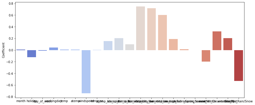
Checking for positive/negative correlation & statisitical significance

Some of the variables have negative correlation like windspeed, atemp_bin_cold, humidity_bin_high, season_Winter, weather_Mist, weather_Rain/Snow. Other variables with -ve sign have a very low -ve value and can be safely ignored.

Similarly, the table shows variables with positive correlation.

	corr = bikeshare_df.corr(method='pearson')
	print('------ Positive/negative correlation with predictor variable(count) --------')
	print(corr['count'])
	print('------------------------------')

view raw b3a369da-9f64-47cb-b6b0-e1274abe97c4 hosted with ❤ by GitHub

------ Positive/negative correlation with predictor variable(count) --------
month                      0.186275
holiday                   -0.004103
day_of_week               -0.045716
workingday                 0.042159
temp                       0.516475
atemp                      0.516624
windspeed                 -0.195128
count                      1.000000
temp_no                    0.429402
atemp_bin_cold            -0.225357
atemp_bin_mild             0.388137
atemp_bin_warm             0.161776
humidity_bin_low          -0.076209
humidity_bin_medium        0.201935
humidity_bin_high         -0.153773
season_Fall                0.071844
season_Spring              0.101960
season_Summer              0.294050
season_Winter             -0.471729
weather_Clear to Cloudy    0.219172
weather_Mist              -0.140658
weather_Rain/Snow         -0.233985
Name: count, dtype: float64
------------------------------

Statistical significance

Statistical significance can be measured using P-values.

more the number of *(stars) and higher the value, the statistical significance would be higher.

Note: Statistical significance assumes linear dependencies.

	from scipy.stats import pearsonr, probplot, norm, shapiro
	import numpy as np

	rho = bikeshare_df.corr().round(2)
	pval = bikeshare_df.corr(method=lambda x, y: pearsonr(x, y)[1]) - np.eye(*rho.shape)
	p = pval.applymap(lambda x: "".join(["*" for t in [0.01, 0.05, 0.1] if x <= t]))
	corr_sig = rho.astype(str) + p
	corr_sig

view raw 5b69c47c-d702-4fdd-a113-daa4651c5d34 hosted with ❤ by GitHub

	month	holiday	day_of_week	workingday	temp	atemp	windspeed	count	temp_no	atemp_bin_cold	atemp_bin_mild	atemp_bin_warm	humidity_bin_low	humidity_bin_medium	humidity_bin_high	season_Fall	season_Spring	season_Summer	season_Winter	weather_Clear to Cloudy	weather_Mist	weather_Rain/Snow
month	1.0***	0.02	0.01	-0.01	0.11***	0.12***	-0.12***	0.19***	0.15***	-0.08**	0.29***	-0.12***	-0.16***	0.03	0.1***	0.4***	-0.11***	-0.05	-0.23***	-0.04	0.01	0.06*
holiday	0.02	1.0***	-0.12***	-0.25***	-0.03	-0.03	0.01	-0.0	-0.02	0.02	-0.07*	0.05	-0.03	0.03	-0.01	0.02	-0.02	-0.03	0.03	0.03	-0.02	-0.03
day_of_week	0.01	-0.12***	1.0***	0.2***	0.03	0.03	0.0	-0.05	0.01	0.01	0.0	0.03	0.02	-0.03	0.02	0.0	0.0	0.01	-0.01	-0.0	-0.03	0.1***
workingday	-0.01	-0.25***	0.2***	1.0***	0.05	0.05	-0.02	0.04	0.05	-0.02	0.06	0.01	-0.03	0.05	-0.02	-0.01	0.01	0.02	-0.03	-0.06	0.05	0.03
temp	0.11***	-0.03	0.03	0.05	1.0***	0.99***	-0.16***	0.52***	0.55***	-0.47***	0.47***	0.58***	-0.15***	0.11***	0.01	-0.22***	0.16***	0.68***	-0.62***	0.12***	-0.1***	-0.06
atemp	0.12***	-0.03	0.03	0.05	0.99***	1.0***	-0.18***	0.52***	0.54***	-0.44***	0.47***	0.58***	-0.17***	0.12***	0.01	-0.21***	0.16***	0.66***	-0.62***	0.11***	-0.09**	-0.07*
windspeed	-0.12***	0.01	0.0	-0.02	-0.16***	-0.18***	1.0***	-0.2***	-0.13***	0.09**	-0.1***	-0.11***	0.28***	-0.13***	-0.1***	-0.14***	0.1***	-0.14***	0.18***	-0.0	-0.04	0.12***
count	0.19***	-0.0	-0.05	0.04	0.52***	0.52***	-0.2***	1.0***	0.43***	-0.23***	0.39***	0.16***	-0.08**	0.2***	-0.15***	0.07*	0.1***	0.29***	-0.47***	0.22***	-0.14***	-0.23***
temp_no	0.15***	-0.02	0.01	0.05	0.55***	0.54***	-0.13***	0.43***	1.0***	-0.17***	0.5***	0.07*	-0.16***	0.03	0.11***	-0.03	0.19***	0.29***	-0.45***	0.01	0.0	-0.03
atemp_bin_cold	-0.08**	0.02	0.01	-0.02	-0.47***	-0.44***	0.09**	-0.23***	-0.17***	1.0***	-0.55***	-0.29***	-0.01	-0.03	0.04	0.34***	-0.08**	-0.41***	0.16***	-0.1***	0.09**	0.03
atemp_bin_mild	0.29***	-0.07*	0.0	0.06	0.47***	0.47***	-0.1***	0.39***	0.5***	-0.55***	1.0***	-0.32***	-0.1***	-0.03	0.12***	-0.08**	0.31***	0.15***	-0.38***	-0.0	0.01	-0.02
atemp_bin_warm	-0.12***	0.05	0.03	0.01	0.58***	0.58***	-0.11***	0.16***	0.07*	-0.29***	-0.32***	1.0***	-0.06	0.16***	-0.13***	-0.23***	-0.13***	0.58***	-0.23***	0.15***	-0.13***	-0.07*
humidity_bin_low	-0.16***	-0.03	0.02	-0.03	-0.15***	-0.17***	0.28***	-0.08**	-0.16***	-0.01	-0.1***	-0.06	1.0***	-0.51***	-0.25***	-0.15***	0.08**	-0.07*	0.14***	0.3***	-0.28***	-0.07**
humidity_bin_medium	0.03	0.03	-0.03	0.05	0.11***	0.12***	-0.13***	0.2***	0.03	-0.03	-0.03	0.16***	-0.51***	1.0***	-0.69***	0.07**	-0.12***	0.11***	-0.06*	0.24***	-0.17***	-0.2***
humidity_bin_high	0.1***	-0.01	0.02	-0.02	0.01	0.01	-0.1***	-0.15***	0.11***	0.04	0.12***	-0.13***	-0.25***	-0.69***	1.0***	0.05	0.08**	-0.07*	-0.06	-0.52***	0.43***	0.27***
season_Fall	0.4***	0.02	0.0	-0.01	-0.22***	-0.21***	-0.14***	0.07*	-0.03	0.34***	-0.08**	-0.23***	-0.15***	0.07**	0.05	1.0***	-0.33***	-0.33***	-0.33***	-0.06*	0.03	0.09**
season_Spring	-0.11***	-0.02	0.0	0.01	0.16***	0.16***	0.1***	0.1***	0.19***	-0.08**	0.31***	-0.13***	0.08**	-0.12***	0.08**	-0.33***	1.0***	-0.34***	-0.33***	-0.02	0.04	-0.04
season_Summer	-0.05	-0.03	0.01	0.02	0.68***	0.66***	-0.14***	0.29***	0.29***	-0.41***	0.15***	0.58***	-0.07*	0.11***	-0.07*	-0.33***	-0.34***	1.0***	-0.34***	0.11***	-0.1***	-0.03
season_Winter	-0.23***	0.03	-0.01	-0.03	-0.62***	-0.62***	0.18***	-0.47***	-0.45***	0.16***	-0.38***	-0.23***	0.14***	-0.06*	-0.06	-0.33***	-0.33***	-0.34***	1.0***	-0.02	0.03	-0.02
weather_Clear to Cloudy	-0.04	0.03	-0.0	-0.06	0.12***	0.11***	-0.0	0.22***	0.01	-0.1***	-0.0	0.15***	0.3***	0.24***	-0.52***	-0.06*	-0.02	0.11***	-0.02	1.0***	-0.94***	-0.23***
weather_Mist	0.01	-0.02	-0.03	0.05	-0.1***	-0.09**	-0.04	-0.14***	0.0	0.09**	0.01	-0.13***	-0.28***	-0.17***	0.43***	0.03	0.04	-0.1***	0.03	-0.94***	1.0***	-0.12***
weather_Rain/Snow	0.06*	-0.03	0.1***	0.03	-0.06	-0.07*	0.12***	-0.23***	-0.03	0.03	-0.02	-0.07*	-0.07**	-0.2***	0.27***	0.09**	-0.04	-0.03	-0.02	-0.23***	-0.12***	1.0***

	count_corr = corr_sig.iloc[:, 7].reset_index().rename(columns={'index': 'Variable', 'count': 'Correlation & Significance'})
	count_corr

view raw e3aa601a-2561-46a5-af27-6e33aa54ca69 hosted with ❤ by GitHub

	Variable	Correlation & Significance
0	month	0.19***
1	holiday	-0.0
2	day_of_week	-0.05
3	workingday	0.04
4	temp	0.52***
5	atemp	0.52***
6	windspeed	-0.2***
7	count	1.0***
8	temp_no	0.43***
9	atemp_bin_cold	-0.23***
10	atemp_bin_mild	0.39***
11	atemp_bin_warm	0.16***
12	humidity_bin_low	-0.08**
13	humidity_bin_medium	0.2***
14	humidity_bin_high	-0.15***
15	season_Fall	0.07*
16	season_Spring	0.1***
17	season_Summer	0.29***
18	season_Winter	-0.47***
19	weather_Clear to Cloudy	0.22***
20	weather_Mist	-0.14***
21	weather_Rain/Snow	-0.23***

	import numpy as np
	from sklearn.model_selection import train_test_split
	from sklearn import metrics
	from sklearn.metrics import r2_score, mean_squared_error, mean_squared_log_error

	def split_dataset(df):
	features = df.columns.values.tolist()
	features.remove('count')

	X = df[features]
	y = df['count']
	yLog = np.log1p(y)
	X_train, X_test, y_train, y_test = train_test_split(X, yLog, test_size=0.3, random_state=101)
	return X_train, X_test, y_train, y_test

	def plot_predictions(y_test, pred):
	sns.scatterplot(x = y_test, y = pred)
	plt.xlabel('Count')
	plt.ylabel('Predictions')
	plt.show()

	sns.distplot((y_test-pred),bins=100, color = 'gray')

	def evaluation(y_test, pred):
	r2 = r2_score(y_test,pred)
	print(f"R2: {r2*100} %")
	print(f"RMSE: {np.sqrt(mean_squared_error(y_test, pred))}")
	print('RMSLE:', np.sqrt(metrics.mean_squared_log_error(np.exp(y_test), np.exp(pred))))

view raw b817c6f9-8973-4ec2-9bbf-01b2bd90d5ef hosted with ❤ by GitHub

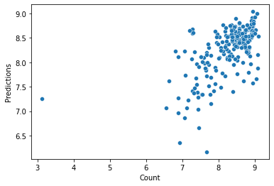
Linear regression without polynomial transformation

X_train, X_test, y_train, y_test = split_dataset(bikeshare_df)

view raw d9230b18-dd76-428e-9b72-91e11ab3a972 hosted with ❤ by GitHub

	from sklearn import linear_model

	linear_regression = linear_model.LinearRegression()
	linear_regression.fit(X_train,y_train)

view raw 852e76dd-25f2-42eb-a0bc-0c57c6b38187 hosted with ❤ by GitHub

LinearRegression(copy_X=True, fit_intercept=True, n_jobs=None, normalize=False)

	plt.figure(figsize = (14,6))
	coeff = pd.DataFrame(linear_regression.coef_, index = X_train.columns, columns = ['Coefficient'])
	sns.barplot(x = coeff.index, y = 'Coefficient', data = coeff, palette='coolwarm')

view raw 40e09a2e-b052-433c-83c9-5976f0c803b5 hosted with ❤ by GitHub

<matplotlib.axes._subplots.AxesSubplot at 0x7fe851c2a828>

png

	plt.figure(figsize = (8,4))
	pred = linear_regression.predict(X_test)
	plot_predictions(y_test, pred)

view raw abaff5a8-89cf-4f33-afe8-ce75cbf8b29d hosted with ❤ by GitHub

png

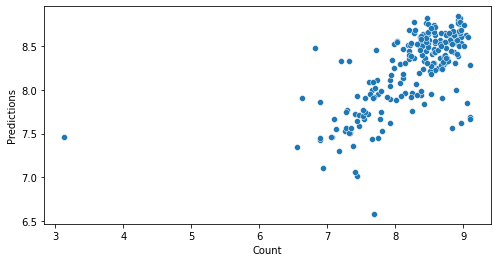
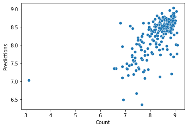
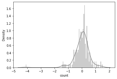
Evaluating predictions

We can evaluate the predictions using Root mean Squared Log Error (RMSLE)

	from sklearn import metrics

	evaluation(y_test, pred)

view raw 0293a085-a6aa-4a36-a1ad-898cb1a0b79d hosted with ❤ by GitHub

R2: 44.029165944830574 %
RMSE: 0.5088707035845853
RMSLE: 0.5071272452091635

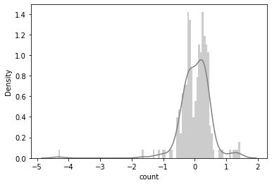
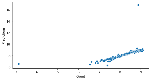
Back to polynomial transformation

Now, that we have seen that without polynomial transformation we get a RMSLE score of 0.507 lets try with the polynomial transformation.

	features = bikeshare_df.columns.values.tolist()

	print(features)

	from sklearn.preprocessing import PolynomialFeatures

	poly_trans = PolynomialFeatures(degree=2)
	data = poly_trans.fit_transform(bikeshare_df[features])

	print(poly_trans.get_feature_names(bikeshare_df.columns))

	bikeshare_df_poly = pd.DataFrame(data, columns = poly_trans.get_feature_names(bikeshare_df.columns))
	print(bikeshare_df_poly.head())

view raw 6691df62-a876-422e-bf1b-f7c8d6b25806 hosted with ❤ by GitHub

     1  month  ...  weather_Mist weather_Rain/Snow  weather_Rain/Snow^2
0  1.0    8.0  ...                             0.0                  0.0
1  1.0    2.0  ...                             0.0                  0.0
2  1.0    6.0  ...                             0.0                  0.0
3  1.0    2.0  ...                             0.0                  0.0
4  1.0   11.0  ...                             0.0                  1.0

[5 rows x 276 columns]

X_train, X_test, y_train, y_test = split_dataset(bikeshare_df_poly)

view raw 38eaaca8-a8eb-4bf3-95a1-9582184d47aa hosted with ❤ by GitHub

	from sklearn import linear_model

	linear_regression = linear_model.LinearRegression()
	linear_regression.fit(X_train,y_train)

view raw 0545cfc8-4a9e-4abd-b19a-dd5cbda10724 hosted with ❤ by GitHub

LinearRegression(copy_X=True, fit_intercept=True, n_jobs=None, normalize=False)

	plt.figure(figsize = (8,4))
	pred = linear_regression.predict(X_test)

	plot_predictions(y_test, pred)

view raw 5f23ad29-0930-469d-bc4c-4dc7d94e4a73 hosted with ❤ by GitHub

png

/usr/local/lib/python3.6/dist-packages/seaborn/distributions.py:2557: FutureWarning: `distplot` is a deprecated function and will be removed in a future version. Please adapt your code to use either `displot` (a figure-level function with similar flexibility) or `histplot` (an axes-level function for histograms).
  warnings.warn(msg, FutureWarning)

png

	from sklearn import metrics

	evaluation(y_test, pred)

view raw 59862dc0-f62d-44da-a960-2c37649e3af9 hosted with ❤ by GitHub

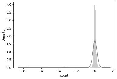
R2: 22.13254677543377 %
RMSE: 0.6002118212313721
RMSLE: 0.5991302674566322

Random forest regressor

X_train, X_test, y_train, y_test = split_dataset(bikeshare_df)

view raw bfd13fdd-e221-40a1-b98c-fdc918ba702d hosted with ❤ by GitHub

	from sklearn.ensemble import RandomForestRegressor
	rfr = RandomForestRegressor(n_estimators= 100)
	rfr.fit(X_train, y_train)

view raw 7cd11d65-ac88-4a44-8ec2-f14d1e27bf22 hosted with ❤ by GitHub

RandomForestRegressor(bootstrap=True, ccp_alpha=0.0, criterion='mse',
                      max_depth=None, max_features='auto', max_leaf_nodes=None,
                      max_samples=None, min_impurity_decrease=0.0,
                      min_impurity_split=None, min_samples_leaf=1,
                      min_samples_split=2, min_weight_fraction_leaf=0.0,
                      n_estimators=100, n_jobs=None, oob_score=False,
                      random_state=None, verbose=0, warm_start=False)

	plt.figure(figsize = (8,4))
	pred = rfr.predict(X_test)

	plot_predictions(y_test, pred)

view raw 39657e9c-ca97-4df0-bec5-d00977648000 hosted with ❤ by GitHub

png

/usr/local/lib/python3.6/dist-packages/seaborn/distributions.py:2557: FutureWarning: `distplot` is a deprecated function and will be removed in a future version. Please adapt your code to use either `displot` (a figure-level function with similar flexibility) or `histplot` (an axes-level function for histograms).
  warnings.warn(msg, FutureWarning)

png

	from sklearn import metrics

	evaluation(y_test, pred)

view raw 9cc2ab9d-de78-4ba2-9e3f-762b0801e017 hosted with ❤ by GitHub

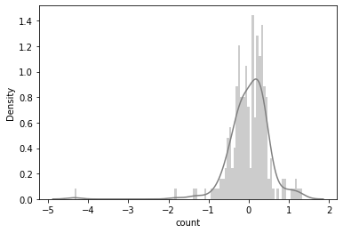
R2: 40.83093585563251 %
RMSE: 0.5232074381024822
RMSLE: 0.5214938879406389

Gradient boosting regressor

	from sklearn.ensemble import GradientBoostingRegressor

	gb = GradientBoostingRegressor(loss ='huber', n_estimators=300, max_depth=5,)

	gb.fit(X_train,y_train)
	ypred = gb.predict(X_test)

	plot_predictions(y_test, ypred)

view raw 892aa1ce-d446-44b2-92c0-df61cd22490c hosted with ❤ by GitHub

png

/usr/local/lib/python3.6/dist-packages/seaborn/distributions.py:2557: FutureWarning: `distplot` is a deprecated function and will be removed in a future version. Please adapt your code to use either `displot` (a figure-level function with similar flexibility) or `histplot` (an axes-level function for histograms).
  warnings.warn(msg, FutureWarning)

png

	from sklearn import metrics

	evaluation(y_test, ypred)

view raw 88db87ea-7745-4f84-8f6b-af92f3fb4aa0 hosted with ❤ by GitHub

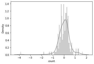
R2: 41.92546239525904 %
RMSE: 0.5183456277546589
RMSLE: 0.5167765321375696

XG Boost Regressor

	import xgboost as xgb
	from scipy.stats import uniform, randint
	from sklearn.model_selection import RandomizedSearchCV

	xgb_model = xgb.XGBRegressor(n_estimators= 300, max_depth=7, learning_rate= 0.18 )

	xgb_model.fit(X_train, y_train)
	ypred = xgb_model.predict(X_test)

	plot_predictions(y_test, ypred)

view raw 05e8b41a-59a2-451e-b0f2-f12fa3223954 hosted with ❤ by GitHub

[06:03:21] WARNING: /workspace/src/objective/regression_obj.cu:152: reg:linear is now deprecated in favor of reg:squarederror.

png

/usr/local/lib/python3.6/dist-packages/seaborn/distributions.py:2557: FutureWarning: `distplot` is a deprecated function and will be removed in a future version. Please adapt your code to use either `displot` (a figure-level function with similar flexibility) or `histplot` (an axes-level function for histograms).
  warnings.warn(msg, FutureWarning)

png

	from sklearn import metrics

	evaluation(y_test, ypred)

view raw 956626ff-d11f-46fc-afc7-3ddf1045444d hosted with ❤ by GitHub

R2: 35.83080957789135 %
RMSE: 0.5448661642271247
RMSLE: 0.5432712054784864

Conclusion

The results for different models are shown in the table below. Clearly linear regression with polynomial transformation performs the best in terms of RMSE score.

Model	R2 Score(%)	RMSE	RMSLE
Linear regression	44.02	0.508	0.507
Linear regression (polynomial)	22.13	0.60	0.59
Random forest regressor	43.28	0.512	0.510
Gradient boosting regressor	43.44	51.1	51.0
XG Boost regressor	25.83	0.544	0.5432

Data Science